
Shear Rate Calculation for Pipe Flow & Tank Agitator Pumping Capacity
Step-by-step hydrodynamic & mixing calculations in different conditions
Question or remark ? Please contact us at contact@myengineeringtools.com
1. Introduction & Pipe Shear Rate Fundamentals
2. Non-Newtonian Fluids & Power Law Models
3. Hydrodynamic Correlations (Mooney-Rabinowitsch, Metzner-Reed)
4. Tank Agitator Pumping Capacity & Pumping Numbers (\(N_q\))
5. Types of Agitators & Recommended Pumping Numbers
6. Interactive Agitator Pumping & Shear Rate Calculator
This technical engineering guide details the methodology to calculate shear rate in a pipe across various rheological models (Newtonian, power-law, slip boundary) and pumping flow capacity (\(Q\)) of agitated vessels using empirical pumping numbers (\(N_q\)).
1. Introduction to Pipe Shear Rate
Shear rate calculation is critical when handling non-Newtonian slurries, polymer melts, or food pastes, because the apparent viscosity directly depends on the local shear rate inside the pipeline.
The shear rate is expressed in \( \text{s}^{-1} \) and quantifies how rapidly adjacent layers of fluid move relative to each other.
When pumping a Newtonian fluid in a circular conduit under laminar flow conditions, the wall shear rate is calculated directly as:
\[ \dot{\gamma}_w = \frac{8v}{d} \]With:
- \( v \) = average linear velocity (\(\text{m/s}\))
- \( d \) = internal diameter of the pipe (\(\text{m}\))
Alternatively, using volumetric flow rate (\(Q\)) and pipe internal radius (\(r\)), the wall shear rate is:
\[ \dot{\gamma}_w = \frac{4Q}{\pi r^3} \]For Newtonian fluids, the wall shear stress (\(\tau_w\)) relates to the wall shear rate simply by the fluid dynamic viscosity (\(\mu\)):
\[ \tau_w = \mu \dot{\gamma}_w \]However, many industrial fluids are non-Newtonian, meaning the apparent viscosity varies with the velocity gradient.
2. Non-Newtonian Fluids & Power-Law Rheology
Non-Newtonian fluids can be characterized as shear-thinning (pseudoplastic), shear-thickening (dilatant), or yield-stress plastic (Bingham/Herschel-Bulkley). For in-depth theory, see our reference on Non-Newtonian Fluids Viscosity.
The classic Ostwald-de Waele Power-Law model relates shear stress to shear rate:
\[ \tau = K \dot{\gamma}^n \]Where:
- \( K \) is the flow consistency index (\(\text{Pa}\cdot\text{s}^n\))
- \( n \) is the dimensionless flow behavior index (\(n < 1\) for shear-thinning, \(n = 1\) for Newtonian, \(n > 1\) for shear-thickening)
The apparent viscosity (\(\mu_{\text{app}}\)) is therefore:
\[ \mu_{\text{app}} = \frac{\tau}{\dot{\gamma}} = K \dot{\gamma}^{n-1} \]Taking the logarithm of both sides enables linear regression from rheometer shear curves:
\[ \log \mu = \log K + (n-1)\log \dot{\gamma} \]The flow index \(n\) equals the slope \(m = \frac{d(\log \mu)}{d(\log \dot{\gamma})}\) plus 1: \(n = m + 1\).
3. Wall Shear Rate Hydrodynamic Correlations
Selecting the appropriate correlation depends on fluid rheology, flow regime (laminar vs. turbulent), and the presence of wall boundary slip:
| Flow Behavior Index \(n\) | Wall Slip? | Recommended Correlation | Engineering Notes |
|---|---|---|---|
| \(n = 1\) (Newtonian) | No | Hagen-Poiseuille (Laminar), Moody / Blasius (Turbulent) | Standard parabolic velocity profile: \(\dot{\gamma}_w = 8v/d\) |
| \(0 < n < 1\) (Shear-thinning) | No | Mooney-Rabinowitsch (Laminar) | Corrects for blunted, plug-like velocity profile |
| \(0 < n < 1\) | Yes | Mooney-Bagley Corrections | Requires experimental capillary tubes of multiple diameters |
| \(n > 1\) (Shear-thickening) | No | Modified Power-Law Correlations | Verify model applicability under elevated shear gradients |
3.1 Mooney-Rabinowitsch Equation (Laminar Flow, Non-Newtonian)
For fully developed laminar pipe flow without slip, the true shear rate at the wall (\(\dot{\gamma}_w\)) is adjusted via the Rabinowitsch correction factor:
\[ \dot{\gamma}_w = \left(\frac{3n' + 1}{4n'}\right) \times \frac{8v}{d} \]Where \(n'\) is the apparent flow behavior index determined at the wall shear stress condition.
3.2 Metzner-Reed Correlation (Turbulent Flow)
For generalized power-law pipe flow, the generalized Reynolds number (\(\text{Re}_g\)) is defined as:
\[ \text{Re}_g = \frac{\rho u^{2-n} d^n}{K 8^{n-1}} \]Where \(\rho\) is density (\(\text{kg/m}^3\)), \(u\) is mean velocity (\(\text{m/s}\)), and \(d\) is pipe inner diameter (\(\text{m}\)). When \(\text{Re}_g > 2,100 - 3,000\), transition to turbulence occurs.
💡 Industrial Best Practices & Rules of Thumb for Piping & Agitation
- Liquid Pipe Velocities: Maintain pump suction piping between 0.8 and 1.5 m/s (2.5–5.0 ft/s) to prevent cavitation, and pump discharge between 1.5 and 2.5 m/s (5.0–8.0 ft/s) for economic pressure drop.
- Impeller Tip Speed Limits (\(v_{\text{tip}} = \pi D N\)):
- Mild Blending / Heat Transfer: 2.5 to 3.5 m/s (500–700 ft/min)
- Solids Suspension: 3.0 to 5.0 m/s (600–1000 ft/min)
- Intense Gas Dispersion / Emulsification: 5.0 to 8.5 m/s (1000–1700 ft/min)
- Tank Turnover Rate: Pumping flow should cycle the entire tank working volume within 0.5 to 2.0 minutes for aggressive blending, or 2 to 5 minutes for general storage agitation: \(\theta_{\text{turnover}} = V_{\text{tank}} / Q\).
- Shear-Sensitive Products: Cell cultures, polymer flocs, and food emulsions typically degrade at shear rates exceeding \(500\text{--}1,000\text{ s}^{-1}\). Use high-solidity hydrofoils with low rotational speeds.
4. Tank Agitator Pumping Capacity Fundamentals
When designing an agitated tank, process engineers must ensure adequate bulk fluid circulation in addition to motor power draw. Tank agitator power calculation is performed using the Power Number (\(N_p\)), while bulk circulation is quantified via the Pumping Number (\(N_q\)).
The pumping capacity (\(Q\)) is defined as the volumetric liquid flow rate passing directly through the impeller sweep area over one second.
In coherent engineering units, the dimensionless pumping number is defined as:
\[ N_q = \frac{Q}{N \cdot D^3} \]Rearranging yields the total agitator pumping flow capacity:
\[ Q = N_q \cdot N \cdot D^3 \]Where:
- \( Q \) = Impeller volumetric pumping capacity (\(\text{m}^3/\text{s}\) or \(\text{ft}^3/\text{s}\))
- \( N_q \) = Dimensionless pumping flow number (-)
- \( D \) = Impeller diameter (\(\text{m}\) or \(\text{ft}\))
- \( N \) = Agitator rotational speed in revolutions per second (\(\text{rev/s}\), where \(N = \text{rpm} / 60\))
When the impeller Reynolds number (\(\text{Re} = \rho N D^2 / \mu\)) exceeds 10,000, the flow regime is fully turbulent, and the pumping number \(N_q\) remains constant regardless of viscosity.
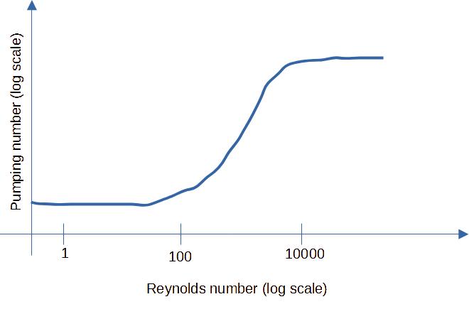
Figure 1: Agitator Pumping Number (\(N_q\)) vs. Reynolds Number (\(\text{Re}\)), illustrating constant asymptotic value for \(\text{Re} > 10^4\).
5. Agitator Types and Recommended Pumping Numbers
Standard industrial impellers are divided into axial-flow (high pumping flow, low shear) and radial-flow (high shear, moderate pumping):
| Impeller Geometry | Flow Direction | Standard \(N_q\) Range (\(\text{Re} > 10,000\)) | Primary Application |
|---|---|---|---|
| Marine Propeller | Axial | 0.40 – 0.60 (Dynamix: 0.5–0.7, Michigan: 0.50) | General blending, rapid turnover in small volumes |
| Pitched Blade Turbine (PBT, 45°) | Mixed / Axial | 0.70 – 0.90 (Hall: 0.79, Michigan: 0.87) | Solids suspension, turbulent bulk blending |
| Hydrofoil Impeller (e.g. A310) | High-Efficiency Axial | 0.55 – 0.73 (Dynamix: 0.6–0.7) | Maximum pumping per unit power, shear-sensitive fluids |
| Flat Blade Turbine | Radial | 0.70 – 1.20 | High shear liquid-liquid emulsification |
| Disk Flat Blade Turbine (Rushton) | Radial | 0.72 – 1.30 (Michigan: 1.30) | Gas-liquid dispersion, aerobic fermenters |
| Hollow Blade Turbine (Smith) | Radial | 0.76 (Hall) | High gas loading without severe power drop |
| Retreat Curve Impeller | Radial | 0.30 (Hall) | Glass-lined chemical reactor vessels |
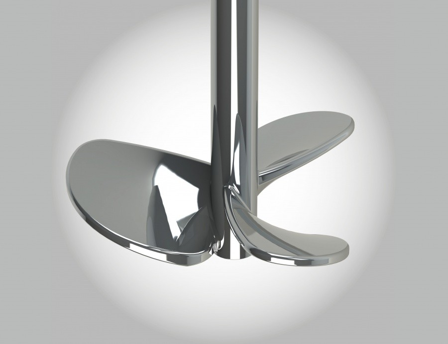
Marine Propeller
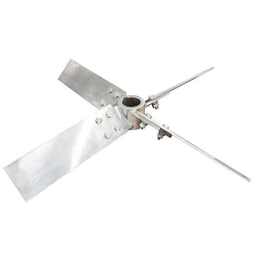
Pitched Blade Turbine
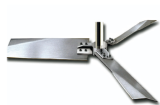
Hydrofoil (A310)
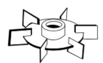
Rushton Turbine
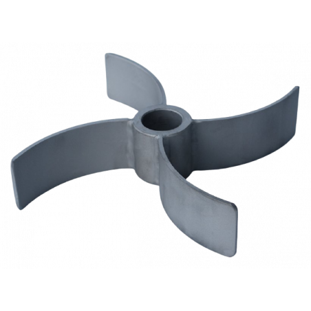
Retreat Curve
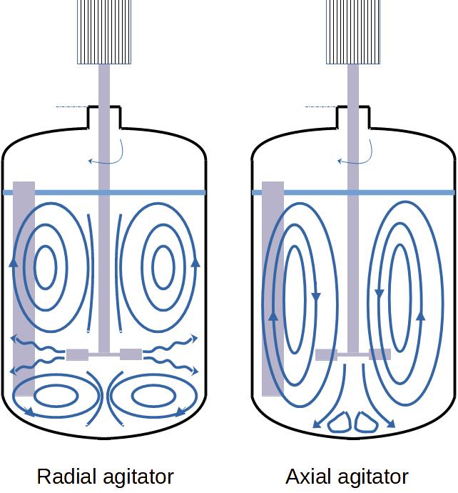
Figure 2: Axial vs. Radial flow circulation patterns generated inside baffled tanks.
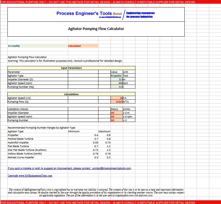
Download the Free Agitator Pumping Flow Excel Calculator
Perform offline equipment sizing, verify turbulent pumping ranges, and audit mixer specifications using our standard spreadsheet template.
6. Interactive Equipment Calculator: Agitator Pumping Flow & Pipe Shear Rate
Equipment Hydrodynamics Sizing Tool
Calculate bulk pumping circulation or pipe wall shear rate with complete dual SI / US Imperial conversion.
Calculation Summary (Agitator Pumping Flow)
Frequently Asked Questions: Tank Agitation & Shear Rate
1. What is the pumping number of an agitator?
The pumping number (\( N_q \)) is a dimensionless parameter that relates the primary fluid pumping discharge (\( Q \)) of an agitator to its rotational speed (\( N \)) and impeller diameter (\( D \)): \[ N_q = \frac{Q}{N \cdot D^3} \] Where \( Q \) is in \(\text{m}^3/\text{s}\), \( N \) in \(\text{rev/s}\), and \( D \) in meters.
2. How is the pumping capacity of an agitator calculated?
When the pumping number (\( N_q \)) is known from vendor catalog or test data, the volumetric pumping capacity is calculated directly as: \[ Q = N_q \cdot N \cdot D^3 \]
3. What are typical pumping numbers for common agitators?
For Reynolds numbers \( \text{Re} > 10,000 \) (turbulent flow): Marine Propeller = 0.40–0.70; 45° Pitched Blade Turbine = 0.70–0.90; High-Efficiency Hydrofoil = 0.55–0.73; Rushton Disk Turbine = 0.72–1.30; Hollow Blade Smith Turbine = 0.76; Retreat Curve Impeller = 0.30.
4. Why are pumping numbers constant at high Reynolds numbers?
At \( \text{Re} > 10,000 \), boundary layers are exceedingly thin and inertial forces dominate the liquid momentum. The flow pattern is fully turbulent and self-similar, so \( N_q \) is strictly determined by impeller geometry.
5. What is the difference between pumping number (\(N_q\)) and power number (\(N_p\))?
The pumping number \( N_q \) quantifies bulk flow circulation generation (\(\text{m}^3/\text{s}\)), whereas the power number \( N_p \) quantifies mechanical power consumption (\(P = N_p \rho N^3 D^5\)). Hydrofoils have moderate \( N_q \) with very low \( N_p \), making them exceptionally energy-efficient for fluid circulation.
6. When must the Mooney-Rabinowitsch correction be used for pipe flow?
The Mooney-Rabinowitsch correction must be applied whenever handling non-Newtonian pseudoplastic (\(n < 1\)) or dilatant (\(n > 1\)) fluids in laminar pipe flow to account for deviation from the classical parabolic Hagen-Poiseuille velocity profile.
References & Standards
[Hall] Rules of Thumb for Chemical Engineers, Hall, Elsevier, 2018, pages 104-105
[Dynamix] Mixing 101: Flow Patterns & Impellers, dynamixinc.com
[Michigan] Chapter 9 Agitation and Mixing, Prof. Faith Morrison, Michigan Tech University
[Steffe] Rheological Methods in Food Process Engineering, Freeman Press