Why do fitting K factors increase drastically in laminar flow?

In laminar flow (Reynolds number Re < 2000), viscous shear force dominates over inertial forces. As fluid velocity and Reynolds number decrease, viscous resistance increases inversely with Reynolds number (K ≈ K1 / Re), causing fitting pressure drop coefficients to become much larger than their turbulent asymptotic values.

What is the Hooper 2-K Method?

The Hooper 2-K method estimates the resistance coefficient K of valves and fittings across laminar and turbulent regimes using equation K = (K1 / Re) + Kt, where K1 accounts for low-Reynolds viscous loss and Kt represents the turbulent contribution adjusted for fitting nominal diameter.

Up to what Reynolds number can standard single K coefficients be used?

Standard turbulent single K coefficients are reasonably accurate for Re > 10,000. Between Re = 500 and 2000, specialized laminar correlations such as Kittredge & Rowley or the Hooper 2-K method must be applied to avoid severe underestimation of pressure drop.

Valves and fittings pressure drop K coefficient (laminar)

Q: What is the Hooper 2-K Method?

The Hooper 2-K method estimates the resistance coefficient K of valves and fittings across laminar and turbulent regimes using equation K = (K1 / Re) + Kt, where K1 accounts for low-Reynolds viscous loss and Kt represents the turbulent contribution adjusted for fitting nominal diameter.

Q: Up to what Reynolds number can standard single K coefficients be used?

Standard turbulent single K coefficients are reasonably accurate for Re > 10,000. Between Re = 500 and 2000, specialized laminar correlations such as Kittredge & Rowley or the Hooper 2-K method must be applied to avoid severe underestimation of pressure drop.

Question or remark ? Please contact us at contact@myengineeringtools.com

1. Definition & Interactive Calculator
2. Pressure Drop Calculation Methods (Hooper & Kittredge)
3. Industrial Best Practices & Design Rules

⚠️ ENGINEERING NOTICE & EDUCATIONAL DISCLAIMER: This interactive calculator is provided exclusively for preliminary estimation and educational purposes. It is not intended for detailed design or equipment procurement without certified vendor rating. No warranty, expressed or implied, is provided, and no liability is assumed.

🧮 Interactive Laminar Fitting K-Factor & Pressure Drop Calculator

Calculate Hooper 2-K resistance factors and pressure loss for viscous flows

Unit System: Metric (SI) Imperial (US)

Select Valve / Pipe Fitting (Hooper 2-K Preset):

Pipe Inside Diameter (mm):

Volumetric Flow Rate (m³/h):

Fluid Density (kg/m³):

Dynamic Viscosity (cP):

Hooper K₁ (Laminar Constant):

Hooper K_∞ (Turbulent Limit):

Quantity of Fittings (N):

Calculation Results

Pipe Fluid Velocity (v): 0.707 m/s

Reynolds Number (Re): 318.3 (Laminar)

Turbulent Factor (K_t): 0.6032

Laminar K Factor (per fitting): 3.116

Total Resistance Coefficient (K_total): 12.464

Total Fitting Pressure Drop (ΔP): 2.81 kPa (0.0281 bar)

Equivalent Pipe Length (L_eq): 1.24 m

1. Definition

The pressure drop caused by piping valves, fittings and other singularities is not the same in turbulent flow and in laminar flow. Turbulent flow have been extensively studied, thus the coefficient are available for many equipment but it is less the case in laminar flow. This page is giving some references from literature for laminar flow. Please consult those references for more details.

2. Pressure drop calculation

K coefficient can reasonably be used until Re=500, below, specific coefficients should be used.

2.1 Kittredge and Rowley

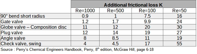
The data of Kittredge and Rowley are reported in many books. They have tabulated the frictional loss coefficients for different fittings and valves and different Reynolds. If the flow is found to be laminar they should be used in pressure calculation instead of the coefficients calculated for turbulent flow

Table 1 : K coefficient for calculation of pressure drop through valves and fittings in laminar flow according to Kittredge and Rowley

Frictional loss coefficient K of valves and fittings in laminar flow - Kittredge and Rowley

2.2 Hooper

As an alternative, the method of Hooper can be used. As most of the data obtained in laminar flow, results are approximate.

The frictional loss coefficient can be calculated from the value in turbulent flow and coefficients to account for laminar flow :

\[ K = \frac{K_1}{Re} + K_t \]

Equation 1 : Hooper approximation for calculation of pressure drop coefficients of valves and fittings in laminar flow

With :
- \(K_1\) = pressure drop coefficient for \(Re=1\)
- \(K_t\) = coefficient in turbulent flow
If unknown, \(K_t\) can be calculated with the following formula where \(K_\infty\) is the coefficient in turbulent flow for a very large diameter:

\[ K_t = K_\infty \left(1 + \frac{0.025}{D}\right) \]

Equation 2 : Calculation of turbulent frictional loss coefficient for Hooper method

Coefficient \(K_1\) can be calculated thanks to the following table.

Table 2 : K1 coefficient for calculation of pressure drop through valves and fittings in laminar flow with the approximation of Hooper

K1 coefficient for Hooper method for calculation of pressure drop coefficients in laminar flow for valves and fittings

💡 Practical Plant Engineering Rules of Thumb & Safety Limits

Laminar Flow Regime Cut-off: Flow is considered laminar when \(Re < 2000\). Between \(Re = 2000\) and \(4000\), flow is in the transition region where pressure drops can fluctuate unpredictably.
Viscous Flow Velocity Limits: For standard viscous liquids (e.g., heavy oils, polymers, syrups), targeted pipe velocities should typically stay between 0.3 to 1.5 m/s (1.0 to 5.0 ft/s) to prevent excessive pump power draw and excessive pressure drops.
Dominance of Fitting Losses in Laminar Regimes: Unlike turbulent flows where pipe friction often dominates long runs, in laminar flows, fittings and small diameter restrictions can generate resistance coefficients \(K > 100\), making fitting losses a primary contribution to line loss.
Hooper 2-K vs Darby 3-K Methods: Hooper's 2-K method provides accurate laminar predictions for standard fittings. For small pipe sizes (\(D < 1 \text{ inch}\) / \(25 \text{ mm}\)), consider cross-checking with Darby's 3-K method for enhanced scaling precision.

Source:

Mecanique et Rheologie des Fluides en Genie Chimique, Midoux, Tec et Docs, 1993, page 348

Perry's Chemical Engineers' Handbook, Perry, McGraw Hill, 2008, page 6-18