Reaction kinetics : rate laws in batch reactor, single reactant

Follow us on Twitter 
Question, remark ? Contact us at contact@myengineeringtools.com

The knowledge of reaction rates is a key data for the design and control of chemical reactors. This page focuses on reaction kinetics in a batch reactor and with a single reactant. It explains how to express and plot the reaction speed for reactions of order 0, 1 and 2.

1. Batch reactor : general reaction speed equation

Assuming that the batch reactor is isotherm, perfectly stirred and of constant volume, the calculation of the mass balance in the reactor shows that the consumption rate of the component A, that is consumed according to the reaction νA = products, is:

\[ r'_A = -\frac{1}{\nu} \frac{d[A]}{dt} \]

r'A = - 1/ν*d[A]/dt

(with ν < 0)

The reaction rate r'A can be expressed as a function of a rate constant k and the concentration of the reactant [A].

\[ k [A]^n = -\frac{1}{\nu} \frac{d[A]}{dt} \]

k[A]ⁿ = - 1/ν*d[A]/dt

with :

n as the order of reaction
ν as the stoechiometric coefficient
[A] as the concentration in reactant A in the batch reactor at time t

2. Order 0 reaction

In the case of a reaction of order 0, the reaction rate is independent of the concentration in reactant A, k[A]⁰ = k

It is then possible to integrate the relation as :

\[ k = -\frac{1}{\nu} \frac{d[A]}{dt} \]

k = - 1/ν*d[A]/dt

\[ k \cdot \nu \cdot dt = - d[A] \]

k.ν.dt = - d[A]

\[ -[A] + [A]_0 = k \cdot \nu \cdot (t - t_0) = k \cdot \nu \cdot t \quad (\text{if } t_0 = 0) \]

-[A]+[A]₀ = k.ν.(t-t₀) = k.ν.t (if t₀ = 0)

\[ [A] = [A]_0 + \nu k t \]

[A] = [A]₀ - k.ν.t

Graphically

It is possible to identify a reaction of order 0 by plotting the concentration over time. If the graph obtained is a line, the reaction of is of order 0 and the slope is -k.ν which allows to calculate the rate constant k if the stoechiometry is known.

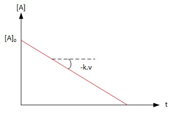
Graph 1 : Graphical identification of a reaction of order 0

3. Order 1 reaction

In the case of a reaction of order 1, the reaction rate is proportional to the concentration in reactant A : k[A] = - 1/ν*d[A]/dt

It is then possible to integrate the relation by rearranging the expression as, a step that is detailed in the batch reactor reaction time calculation guide.

\[ -\frac{d[A]}{[A]} = \nu k dt \]

- d[A]/[A] = k.ν.dt

and integrate as :

\[ \ln\left(\frac{[A]_0}{[A]}\right) = -\nu k (t - t_0) = -\nu k t \quad (\text{if } t_0 = 0) \]

ln ([A]₀/[A]) = k.ν.(t-t₀) = k.ν.t (if t₀ = 0)

\[ \ln\left(\frac{[A]_0}{[A]}\right) = -\nu k t \]

ln ([A]₀/[A]) = k.ν.t

Graphically

It is possible to identify a reaction of order 1 by plotting ln ([A]₀/[A]) over time. If the graph obtained is a line, the reaction of is of order 1 and the slope is k.ν which allows to calculate the rate constant k if the stoechiometry is known

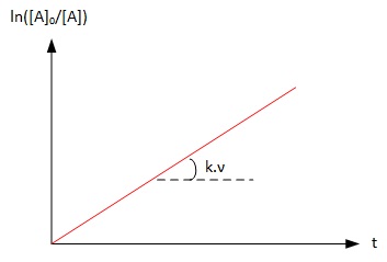
Graph 2 : Graphical identification of a reaction of order 1

4. Order 2 reaction

In the case of a reaction of order 2, the reaction rate is proportional to the square of concentration in reactant A : k[A]² = - 1/ν*d[A]/dt

It is then possible to integrate the relation by rearranging the expression as :

\[ -\frac{d[A]}{[A]^2} = \nu k dt \]

- d[A]/[A]² = k.ν.dt

and integrate as :

\[ \frac{1}{[A]} - \frac{1}{[A]_0} = -\nu k (t - t_0) = -\nu k t \quad (\text{if } t_0 = 0) \]

1/[A]-1/[A]0 = k.ν.(t-t₀) = k.ν.t (if t₀ = 0)

Graphically

It is possible to identify a reaction of order 2 by plotting 1/[A] over time. If the graph obtained is a straight line, the reaction of is of order 2 and the slope is k.ν which allows to calculate the rate constant k if the stoechiometry is known

Graph 3 : Graphical identification of a reaction of order 2